- The idea of pre-compiled ML models as functions
- Process of starting with ML on Snowflake
- Discovering how to train the model
- Setting up the model for re-training on new data
- Pitfalls when using the current version of models
Most people like simplicity (source:https://www.linkedin.com/pulse/20140620200653-298076-10-favorite-quotes-on-simplicity/). But setting up a forecast model, might not be categorised as a trivial or simple task for all analysts. A simple forecast should take into account, where a dividing line should be between what the user can provide, and what the forecast model should include. Here I will guide the reader through the process of how to utilise a single series forecast model, that only asks for the data a user is actually able to provide: time-series and prepared data values in a “sliced” tabular format.
From recent Snowflake announcements, a new set of machine learning (ML) features is now available in general availability (GA). This means all new accounts can make use of a pre-compiled and standardized way of training models in Snowflake. The provided ML functions are of quite a general type, suitable for base models/PoC’s, so make use of them accordingly.
This article will introduce the concept, and make demoing available. The demo will end up creating forecast predictions with slice variations as:
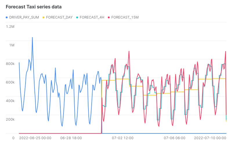
The above graphic shows three trained forecast models, on the same data, but in different slicing: daily, per four hours or every 15 minutes.
The idea of pre-compiled ML models as functions
To lower the bar for implementing ML, Snowflake pre-compiled a group of functions for all users, and these models can be taken as “off the shelf” models, similar to how a user would develop Snowpark python functions, and call them within SQL statements. This approach will be suitable for a broad range of simpler use cases, where ML would usually not be the first tool in the problem solving stack. In my opinion, this opens up new ML applicability and can add a statistical basis for decision making on data, and place it directly in the hands of analysts and managers. This group is already the target for quite a large chunk of Snowflake’s market approach.
Though data scientists will probably claim that this class of functions lacks explainability as well as transparency in its algorithmic design. This is indeed a point, but not all enterprises or employees have access to their own data science department, and would like a shorter time to market for analyses. For a single series forecasting that are not pushing statistical boundaries, the provided gradient boost algorithm (xgboost) will likely prove to be sufficiently detailed.
My guess is that Snowflake gained insight into what their customers are looking for, but also have a need of broadly proving their platform to take on analytical ML workloads in their well known simple fashion.
Process of starting with ML on Snowflake
The basic process for making use of an ML function is the following:
- Prepare time-series data, sliced/grouped into suitable intervals. Store the data object with only data relevant for a model, this means:
- Object contains only the timestamp and the target column.
- Slicing data, means that all data points are represented in a unique window slices, use TIME_SLICE and GROUP BY function in Snowflake SQL.
- Multiple views slicing data differently can exist in parallel, this is done by creating different TIME_SLICE configurations in views/tables.
- Based on prepared data, a FORECAST model is trained to predict:
- CREATE OR REPLACE FORECAST DB.SCHEMA.MODELNAME (INPUT_DATA => SYSTEM$REFERENCE(‘VIEW’, ‘NAME’), TIMESTAMP_COLNAME => ‘TIME_COLUMN’, TARGET_COLNAME => ‘COLUMN_TO_PREDICT’)
- If multiple slicings of data have been prepared, repeat step 6 on each.
- Each forecast model can now be called by its Snowflake object name:CALL MODELNAME!FORECAST(FORECASTING_PERIODS => 100);
- This call create time-series data using forecast model with the trend.
- Store the predictions in separate persistent or temporary table. CREATE TABLE “NAME” AS (SELECT * FROM TABLE(RESULT_SCAN(-1)));
- Use predictions to visualise trends by overlaying existing data. SELECT “TIMESTAMP” as “TS” , “SOURCEVALUE” , NULL AS “FORECAST” FROM “SOURCE_TABLE” UNION SELECT TIME_SLICE(“TS”, 1, HOUR)::TIMESTAMP_NTZ , NULL AS “SOURCEVALUE” , SUM(FORECAST) AS “FORECAST” FROM “FORECAST_TABLE” GROUP BY TIME_SLICE(“TS”, 1, HOUR)::TIMESTAMP_NTZ;
- If you have a dual-column data output from your overlay, click “Chart”, and add your forecast column to the visualisation.
If you trust the released ML functionality, and do not need additional explainability from algorithm tweaking or weighing, then you will at this point have a trained prediction model.
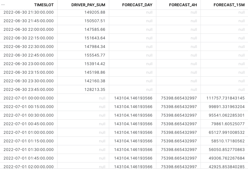
Depending on how many forecasting periods you decided to predict, and how you choose to compare the historic with predicted, you will have something like this:
Once predictions are working, a training/test split can be conducted, and quality metrics of the trained model can be derived of how well it predicts. To perform this test, train the model on only a part of the data, and calculate the deviation from each prediction
Discovering how to train the model
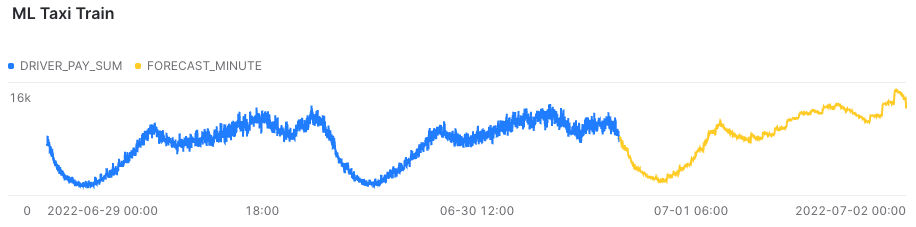
The responsibility of slicing your timescale, and setting up the parameters to use as input data, lies entirely with the analysts who know the data set. To gain some resemblement of your options, I would recommend training a smaller fleet of models on sliced subsets of the source data. E.g. per day, per hour and minute. The above graphic is made from a minute granularity, which in this case seems way too detailed, though presents itself beautifully.
While training multiple models, the analyst becomes familiar with the tool, and the various combinations of how time series slicings can compare each prediction.
Setting up the model for re-training on new data
Depending on use case, this interval is application-specific. But a rule of thumb would be that a lot more data should be available before retraining.
When the ideal slicing approach has been selected, make sure the data pipeline is stable and will contain the updated records when available. When this is done, select a regular interval where you would like the model to be retrained, and schedule this by placing step 2, in a Snowflake task during off-hours. Small tips:
- Construct your data source, so base views will reflect updated data.
- Expose an object that contains both historical and forecasted data.
- Use your favourite visualization tool to overlay the two time series.
Snowsight can present data natively, though additional tweaks are limited. The visualisation below, shows blue historical data, and two trained forecast models; a green with data sliced into 4 hour slots, and a yellow where the slicing is done for each day:
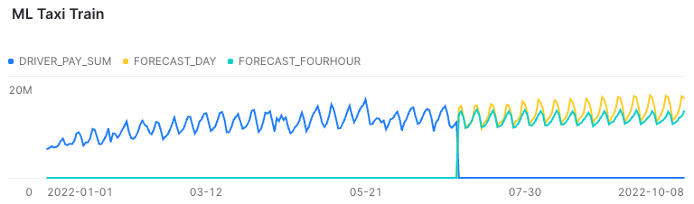
Short term predictions are similar, but only the daily sliced seems to take an overall steady growth into consideration. They are trained on the same data points, just grouped differently for training. Cost of training were done on x–small Snowflake warehouse:
- Green/four hour took around 6 minutes to train.
- Yellow/daily took around 2 minutes to train.
The total of 8 minutes training time amount to less than one euro/dollar in training time, depending on your Snowflake plan. So the initially provided credits by Snowflake, should be more than sufficient in finishing a PoC.
Pitfalls when using the current version of models
A few important topics to mention, to avoid pitfall when designing a prediction model using native Snowflake ML functions:
- All namespaces seem to currently be required in UPPERCASE.
- Create a view for slicing/aggregations, timestamps must be unique.
- Timestamps must not have large gaps, and adhere to “cleaned data”.
- Regular sized warehouses can perform the training for smaller data sets, but warehouses of the SNOWPARK type will not run out of memory for training on larger datasets (for detailed minute-sliced training, I ended up with ~1 M rows, which required around 50 minutes on a medium Snowpark optimized warehouse ~6 Snowflake credits total)

