Algorithm No. 5 – Understanding the “k-nearest neighbours” method

The k-nearest neighbours (k-NN) algorithm is relatively simple to understand. First, you need to know that it is a supervised learning algorithm that allows us to solve not only a classification problem, but also a regression problem.

As a reminder, supervised learning is when an algorithm needs labelled input data (i.e. inputs with a label) and output data (i.e. data that the algorithm will have to predict later).

The idea is as follows: in a learning phase, the algorithm must be trained to learn the relationship between the data inputs and outputs.

This is a key point. In fact, supervised learning is based on the organisation of data according to a series of {input-output} pairs.

Once the algorithm has been trained, it can predict an output
value, solely on the basis of the input values.

The k-nearest neighbours method and its principles

Once an algorithm learning phase has been completed, the algorithm is able to make a prediction based on a new unknown observation by finding the observation that is nearest to it in the training data set.

The algorithm then assigns the label of this training data to the new observation, which was previously unknown.

The k in the formula “k-nearest neighbours” means that instead of just the nearest neighbour of the unknown observation, a fixed number (k) of neighbours in the training data set can be considered.

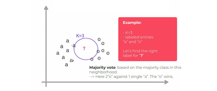
Ultimately, we can make a prediction based on the majority class in this neighbourhood.

This principle may seem complicated to explain, but take a look at the example below which simply illustrates the general idea of this method.

A simple illustration of the algorithm’s principle of operation :

Let’s find the K nearest neighbors of the unknown observation “?”

In summary, the steps of the algorithm are as follows: From the input data:

• A definition function for the distance (also known as a similarity function) is selected between observations. (We will come back to this in the next paragraph.)
• We set a value for “k,” the number of nearest neighbours.

Pseudo code :

We must do the following for a new unknown input observation for which we want to predict the output variable.

• Step 1 – Calculate all the distances between this observation and the other observations in the data set.
• Step 2 – Select the observations from the data set which are the “nearest” to the predicted observation.

Note: To determine whether one value is “nearer” than another, a distance calculation-based similarity function is used (see the next paragraph).

• Step 3 – Take the values of the selected observations:

If a regression is performed, the algorithm will calculate the average (or the median) of the values of the selected observations.
If a classification is performed, the algorithm will assign the label of the majority class to the previously unknown data.

• Step 4 – Return the value calculated in step 3 as the value that was predicted by the algorithm for the previously unknown input observation.

For this algorithm, the choice of the number (k) and the choice of the similarity function are steps which can cause the results to vary greatly.

Metrics for evaluating the similarity between observations

As we have just said, to measure the proximity between observations, a similarity function must be imposed on the algorithm.

This function calculates the distance between two observations and estimates the affinity between the observations like this: “The nearer two points are to each other, the more similar they are.”

However, this trivial statement comes with some mathematical nuances, and there are many similarity functions in related literature.

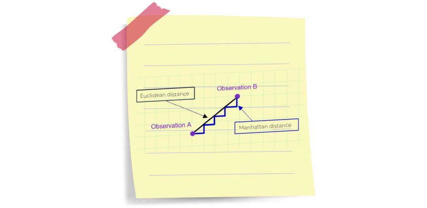
Euclidean Distance is one of the best-known similarity functions. We used this function in the example above.

It is the most intuitive similarity function because it formalises the idea of distance – the straight line distance between two points in space.

Manhattan Distance (also known as Taxicab Geometry) corresponds to a movement at a right angle on a chessboard.

If you are interested, I invite you to look at the mathematical definitions of other metrics such as the Minkowski Function, the Jaccard Function, the Hamming Distance, the Levenshtein Distance, the Jaro Metric, or even the Jaro-Winker Distance.

You need to know that the distance function is generally chosen according to the types of data that we are handling and the mathematical or physical meaning of the problem to be solved. The Euclidean Distance is a good choice to start with for quantitative data (e.g.: height, weight, salary, turnover, etc.), as it is very schematic.

The Manhattan distance can be interesting for data that are not of the same type (e.g. data that have not been put on the same scale). Also, I strongly advise you to deepen your subject knowledge in order to master the classic use cases of the various similarity functions, according to the problem to be solved.

Your turn to code… (Python)

This paragraph provides some elements to help you to code the algorithm yourself. All of the machine learning models in scikitlearn are implemented in their own classes, which are called the Estimator classes.

The class for the k-nearest neighbours algorithm is KNeighboursClassifier, from the neighbours module.

Before we can use the template, it needs to be instantiated as follows:

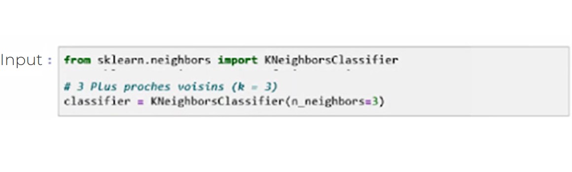
In our example, the classifier object encapsulates the algorithm that will be used to create the model from the training data, as well as the algorithm that will make predictions for new observations.

To create the k-NN model, we must first split the data into 2vdatabases: one for training the algorithm, and one for testing thevperformance obtained.

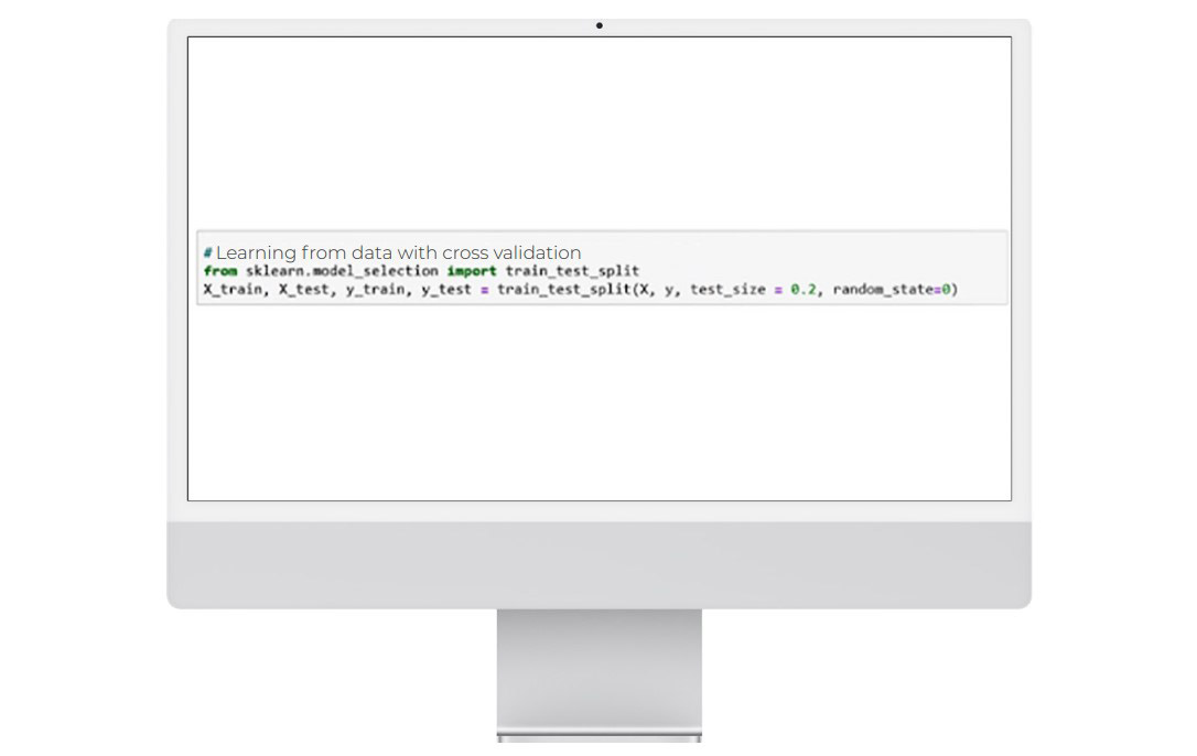
Note: test_size = 0.2 = 20% gives the size of the test database, i.e. 20% of the initial data sample.

Next, we use the fit method of the classifier object, which takes as arguments the training dataset X_train and the test dataset y_train.

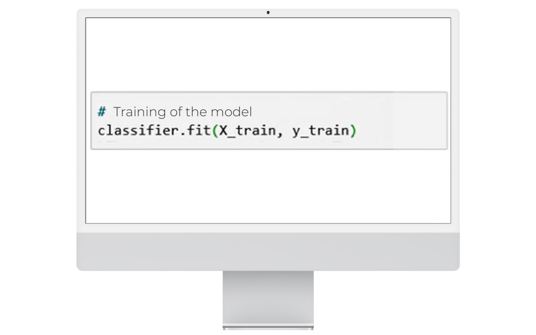
The fit method returns the k-NN object itself.

The default algorithm configuration is as follows:

KNeighboursClassifier (algorithm=’auto’, leaf_size=30, metric=’minkowski’, n_jobs=1, n_neighbours=3, p=2, weights=’uniforms’)

You will notice that all the parameters except for the number of nearest neighbours have their default value set to n_ neighbours=3.

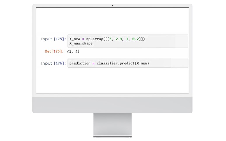
To make a prediction about new unknown data, we create a vector that contains the known input data. The X_new vector is below.

We will then use the predict method of the classifier object.

The limitations of the K-nearest neighbours algorithm

Although the operation of the nearest neighbours algorithm is easy to understand, the main drawback of the method is its cost in terms of complexity. Indeed, the algorithm searches for the k-nearest neighbours for each observation. Therefore, if the database is very large (a few million rows), the calculation time can be extremely long. Special attention must therefore be paid to the size of the input data set.

Another focal point: the choice of similarity function can lead to very different results between models.

It is therefore recommended to create a rigorous state of the art to better choose the similarity distance according to the problem to be solved. Above all, it is recommended to test several combinations to estimate the impact on the results.

Despite everything, remember that if the k-NN algorithm is interesting from a didactic point of view, it is almost never used as it is by data scientists.