
The first chapter of this didactic E-book is about one of the simplest algorithms: the decision tree. A decision tree allows you to use your data to determine clear business rules, according to a target variable that you are seeking to explain. It is rarely used unaltered in machine learning, and is an elementary and essential tool that you must master to understand the algorithms that we will see later: the random forest (Algorithm No. 2) and the isolation forest (Algorithm No. 3).
Working principle
A decision tree makes it possible to make a target variable stand out from other, so-called explanatory, variables.
From a mathematical perspective: given a matrix (X) with m observations and n variables, associated with a vector (Y) to be explained, a relationship between X and Y must be found.
To do this, the algorithm will seek to divide the individuals into groups of individuals that are as similar as possible in terms of the variable to be predicted.
As a result, the algorithm produces a tree that reveals hierarchical relationships between the variables. It is therefore possible to quickly understand the business rules explaining your target variable.
Construction of rules
The decision tree is an iterative algorithm which, at each iteration, separates the individuals into k groups (generally k=2 or a “binary tree”), to explain the target variable.
The first division (or “split”) is achieved by choosing the explanatory variable that will allow the best separation of individuals. This division creates sub-populations corresponding to the first node of the tree.
The splitting process is then repeated several times for each sub-population (previously calculated nodes), until the splitting process ends.
What are your chances of being accepted for a loan at the bank?
Let’s take a look at a specific case to illustrate all of the above. The diagram below helps us to understand the likelihood of being accepted for a bank loan. This is a hypothetical example to demonstrate the principle of reading a decision tree. Imagine that a manager of a large bank wants to know their own rules for accepting or not accepting a bank loan on the basis of the customer’s profile.
To do this, they appoint an advisor, who is responsible for interviewing customers. This adviser (who is something of a statistician at heart) summarises the results for the manager by proposing the decision tree below.
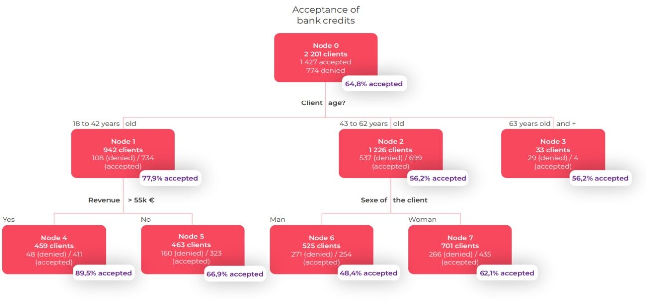
Let’s take a closer look… In the roots of the tree, 2,201 customer files are under review.
Of these files, 1427 will be accepted (64.8%) and 774 will be rejected (35.2%). The explanatory variable that best separates the accepted files (our target variable) from the other files is customer age. Therefore, among 942 customers aged between 18 and 42 years (42.8% of all customers), the credit acceptance rate reaches 77.9% (i.e. 734 customers); while among the 33 customers aged 63+ years, the credit acceptance rate is just 12.1%. The main variable separating the population of customers aged between 18 and 42 years (Node 1) is income. As you can see, the 459 customers with an annual net income above EUR 55K have a credit acceptance rate of 89.5%.
Among customers aged between 43 and 62 years, the main explanatory variable for credit acceptance is gender. Thus, the rate of acceptance of a loan is 62.1% for women, compared to 48.4% for men in the same age group.
The limitations of The Decision Tree
Decision trees can sometimes lead to overfitting. This means that although the algorithm finds a rule that seems perfect
for understanding and describing the data, this rule cannot be generalised. Worse still, in some cases, it is possible that the found rule may change drastically if a few more observations are added to your initial data.
Going a step further
There are a few key questions that you should ask yourself when creating a decision tree.
- Which explanatory input variables should you choose to create your tree? You will need to explain a target variable in terms of other variables. Try to find a causal process in your data (is there a causal relationship between the different variables in your data?).
- How can you process continuous data (e.g.: the height of an individual, the price of a property, etc.) and qualitative data (e.g.: the socio-professional category, etc.)? You need to pre-process the variables and select the decision tree model that works best.
- How can you define the optimal size of a tree? You have to think about pruning the tree (cutting it to a certain height). Indeed, a tree that is too profound (i.e. with lots of nodes) is always synonymous with overfitting.
To continue answering these questions, find out more about the three algorithms of the decision tree family: CHAID, CART and C4.5.
To summarise…
If you fully understand how this first algorithm works, you will easily understand the set methods which put several trees into competition, in particular the random forest (Algorithm No. 2) and the isolation forest (Algorithm No. 3).

The decision tree is easy to understand. With other algorithms, however, a compromise between interpretability and performance is needed.

