
The random forest is a vital algorithm in machine learning. It is also known as a “random decision forest.” Suggested by Leo Breiman in 2001, this algorithm is based on the grouping of multiple decision trees. It is fairly intuitive and easy to train, and it produces generalisable results. The only downside is that the random forest is a black box that gives results that are difficult to read, i.e. not very explanatory.
Nevertheless, it is possible to limit this by using other machine learning techniques. This will be the focus of Algorithm No. 7, LIME – a key algorithm for making an explanatory model.
Random forest – working principle
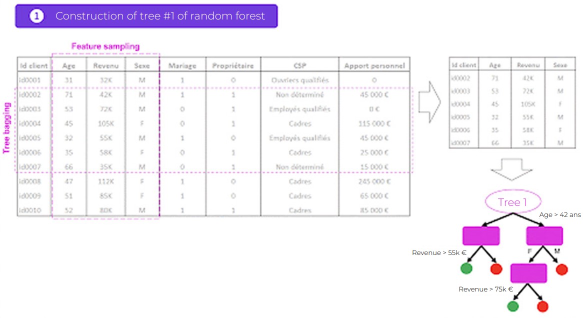
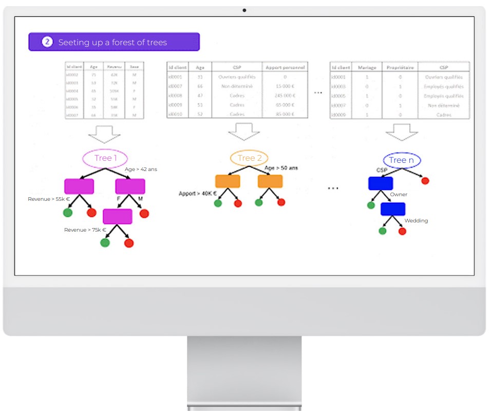
A random forest is made up of a set of independent decision trees.
Each tree has a partial vision of the problem due to a double random selection:
- random selection with replacement of observations (rows of your database). This process is known as tree bagging.
- random selection of variables (columns of your database). This process is known as feature sampling.
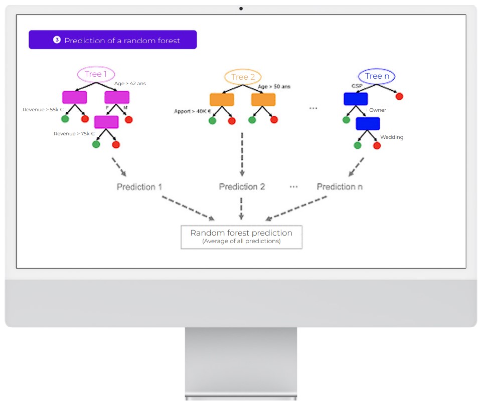
All of these independent decision trees are ultimately put together. The prediction made by the random forest for unknown data is therefore the average (or the vote, in the case of a classification problem) of all the trees.
The basic idea of this algorithm is quite intuitive. For example, if your credit application is rejected by your bank, chances are that you will consult one or more other banks. Indeed, a single opinion is not usually enough to make the best decision.
The random forest works on this same principle. Rather than having a complex estimator which is capable of doing everything, the random forest uses several simple estimators (of lower individual quality). Each estimator has a fragmented view of the problem. All of these estimators are ultimately brought together to obtain a global view of the problem. The combination of all these estimators makes the prediction highly efficient.
Genesis of the algorithm
The major flaw of the decision tree is that its performance is highly dependent on the initial data sample. For example, the addition of some new data to the knowledge base can radically modify the model and change the results.
To fight against this flaw, we can use a multitude of trees – a forest of trees! – hence the name “random forest.” The term “random” comes from the random double draw process that is applied to each tree, in relation to both the variables and the observations.
Practical illustration of the algorithm, A formula to remember:
Random forest = tree bagging + feature sampling.
Tree bagging
“Bagging” is short for “bootstrap aggregation.” It is a process of randomly selecting observation samples (rows of data),
determined by 3 key steps:
- Constructing n decision trees, by randomly selecting n
observation samples. - Training each decision tree;
- To make a prediction on new data, each of n trees must be
used, and the majority is determined from n predictions.
Feature sampling
It is a process of randomly selecting variables (columns of data). By default, n variables for a problem with n variables in total are selected from the root of the decision tree.
Going back to the previous example of credit acceptance, the basic idea of feature sampling is to ask each bank to study your loan application based on limited access to customer information. One bank will make its decision on the basis of only having, for example, access to information relating to the age, CSP and annual income of the customer. Meanwhile, another bank will only have access to information relating to the marital status, gender and current credit rating of the customer.
This process makes it possible to weaken the correlation between the decision trees that could interfere with the quality of the result. In statistics, we say that feature sampling makes it possible to reduce the variance of the data set created.
Split/division criteria
As you know, a decision tree creates sub-populations by successively separating the leaves of a tree.
There are different separation criteria for constructing a tree:
- The Gini criterion organises the separation of the leaves of a tree by focussing on the class most represented in the data set. This must be separated as quickly as possible.
- The entropy criterion is based on the measurement of the prevalent disorder (as in thermodynamics) in the population studied. The construction of the tree aims to lower the global entropy of the leaves of the tree at each stage.
To summarise…
If you understand how the random forest algorithm works, you are ready to discover gradient boosting, which is also an ensemble method.
In the next chapter, you will find out how forest isolation works. This is a modern algorithm, and one of the most frequently used in anomaly or fraud detection cases.

The random forest performs better than the decision tree. It is often used in machine learning competitors, and remains a model that is difficult to interpret.

