Algorithm No. 4 – Linear regression to understand the main principles of machine learning

Many people think that linear regression is straightforward and that it is simply a question of finding a straight line through a scatter plot. They are wrong! We can even say that linear regression is a deceptively simple model. Let’s find out why together.

Modelling well means modelling a phenomenon based on the simplest possible – and most easily interpretable – law. With this in mind, we are going to present the theoretical steps with which to analyse the implementation of a linear model for calculating the life of a mechanical component, in order to optimise the preventive maintenance of our customer.

We have decided to maintain a statistical approach, but mathematical formulae are nothing to be afraid of! This booklet is intended for the general public, and we hope that it will be a good way for you to understand in detail some fundamentals of machine learning.

The best linear regression model can be built by following three key steps:

1. Start by defining a cost function. This is a mathematical function that measures the errors we make when approximating data. It is also known as model-induced error.
2. To minimise this cost function, we must find the right parameters of our model to minimise the modelling error.
3. Select a method of resolving the problem. There are two methods:
   • a digital resolution method, gradient descent;
   • an analytical method, the “least squares” method.

Step 1: Preparation of the cost function.

To create a cost function, we must start by defining an assumption function.

This hypothesis can be summed up as follows: the model depends on a set of n input variables, labelled x1, x2, … xn. (These input variables correspond to the known data. For example, the number of inhabitants of a geographical area, the salary of an employee, or any other known variable.)

These input variables will influence an unknown target variable (Y), which we are seeking to predict.

From a mathematical perspective, we seek to determine the best hypothesis function which will make it possible to find an approximate linear relationship between the input variables and the target variable (Y).

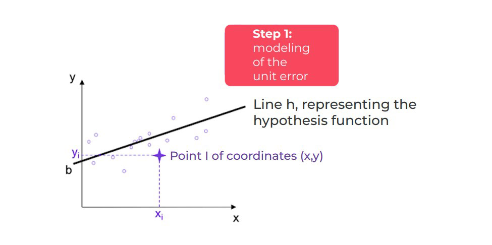
Hypothesis function h

To simplify the approach, we take the simplest case of univariate linear regression. In this case, linear regression applies to a single input variable, and the hypothesis function (h) is written: h(X) = a x + b.

Our challenge is then to find the best approximation, i.e. the best pair (a, b) so that h is as near as possible to all of the points of our data. In other words, we will determine from the data the best linear relationship between the input value (X) and the target variable value (Y), by training the hypothesis function (h).

This hypothesis function is therefore a function that demonstrates the error between the prediction of the model and the actual data.

The hypothesis function assigns to each point X a value defined by h(xi), which is more or less the same as the target variable (yi). We can therefore determine the margin of error for xi as follows: h(xi) – yi. Each margin of error can be either positive or negative. Consequently, the sum of the margins of error may offset each other. It is, therefore, necessary to ensure that the contribution of each error is systematically penalised. The margin of error is then squared (see figure below).

Principle of the algorithm

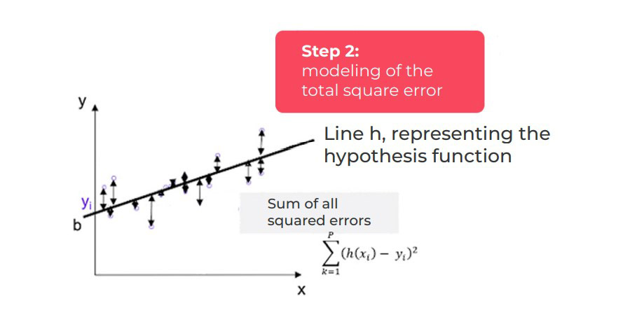
We find the sum of all the unit errors for all the data points, to determine a quadratic error (squared error):

The cost function is then determined by weighting the sum of the squared errors by the number of points p in the learning base:

In our univariate linear regression case, the cost function is determined as follows:

The values of X and Y are given. In terms of its construction, cost function C is a function of the parameters of the hypothesis function (h). And, as shown in the figure above, the parameters of C define an affine line with:

• b, the ordinate at the origin of function h;
• a, the leading coefficient (or slope) of straight-line h.

Note: the same principle applies for multiple linear regression (i.e. linear regression with n input variables).

Step 2: Minimisation of the cost function.

Determining the best parameters (a, b) for the hypothesis function (h) comes down to finding the best straight line – the one that minimises the sum of all unit errors.

From a mathematical perspective, it is a matter of finding the minimum of the cost function.

Squaring the sum of the unit errors does two things:

• On the one hand, it ensures that the cost function is appropriately penalised by each unit error. Indeed, all errors are positive.
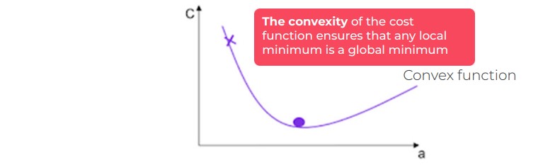
• On the other hand, it guarantees that the cost function is convex (if the cost function admits a minimum, this minimum is the global minimum of the function). We will outline the notion of convexity (see below).

We will also introduce the numerical method of gradient descent, which is used to mathematically find the minimum of the cost function, i.e. the best pair (a, b).

It is an iterative method that can be summed up as follows: if you drop a ball from the top of a hill, the ball will take the best slope at all times as it rolls to the bottom of the hill. The convexity of the cost function corresponds to the fact that we are certain that the hill is not uneven, with up-slope areas.

The mathematical formulation of this gradient descent problem is written as follows:

Step 1: Initialisation of the pair
Step 2: Iteration until convergence:

In each iteration, the best slope is found with our function C, which goes over the iterations toward the minimum of the cost function.

The major problem lies in the case of a non-convex cost function. Indeed, in this case, it may be that according to different initialisations of the descent of the gradient, we converge towards a local minimum for C.

The convexity of the cost function makes it possible to overcome this problem, as any local minimum is the global minimum of the function (refer to the figure below for a better understanding).

Case of a non-convex cost function

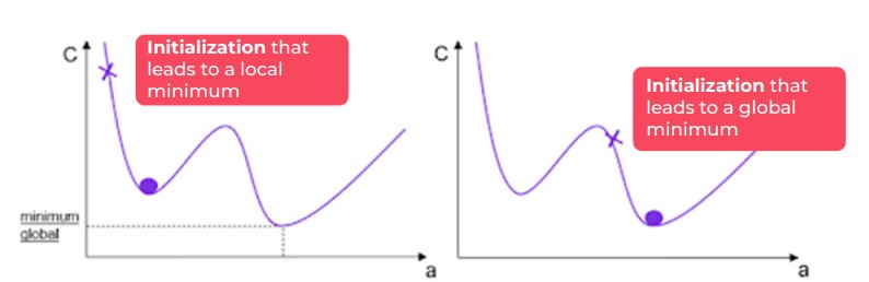
Case of a convex cost function

In the gradient descent formula above, the speed of convergence is determined by the factor α in front of the partial derivative C. This factor is called the learning rate, and represents the speed of modification of each parameter during each iteration.

• The larger α is, the greater the modification of the parameters between two successive iterations (therefore, the greater the probability of “missing” the minimum or of diverging).
• Conversely, the smaller α is, the more likely we are to converge to the minimum (in contrast, the convergence process takes longer).

Gradient descent is the numerical resolution approach to finding a solution to the modelling problem. This method makes it possible to find, in an iterative way, the best model that minimises the error by seeking the best slope up to the global minimum of the cost function.

This method is particularly suitable for large volumes of data, and makes it possible to reach a solution as quickly as possible.

There is another approach: an analytical approach.

This approach involves mathematically solving linear regression. Without going into too much mathematical detail, the so-called least squares method provides an analytical solution to a problem. If you want to know more, a form of analytical resolution for linear regression is written like this:

It’s up to you to elaborate on this, if you need to.

And in practice…

• One of the delicate points of the implementation of a linear regression model comes from the instability of the prediction when faced with the integration of new observations in the data (in other words, the coefficients of each explanatory variable can change drastically if a few additional observations are added to the data),
• It is not usually easy to choose the explanatory input variables to take into account in the model. Questions must then be asked about the nature of the process between the variables. What are the causes for, and effects of, including a specific variable in the model? Immutable relationships between variables must also be found. (These are like the laws of physics, which are universal and therefore do not change – think of the laws of attraction, vibration, transmutation of energy, etc.)
• An additional step of normalising the input variables is vital in the case of multivariate linear regression. This normalisation involves transforming all the variables at the input of the model so that they will evolve on the same scale (to enable the gradient descent algorithm to work correctly),
• The linear model is not suitable for all the physical phenomena involved (e.g.: the phenomena of thermal heating are generally modelled by quadratic relations between electrical and physical measurements). If the phenomenon cannot be modelled by a linear relationship between input and target variables, it is then necessary to find a polynomial function. (But in this case, beware of overfitting – i.e. finding false relationships in your data!)
• Remember the positive points of the linear model: it is an interesting approach because the model is simple to explain to businesses, and the model is explanatory (the coefficients of each normalised variable indicate the importance of the variable in the relationship).

To summarise…

We have seen that linear regression allows you to familiarise yourself with the main principles of constructing a machine
learning model. In a later chapter, we will look at how to improve the stability of linear regression models by penalising LASSO, Ridge or ELASTIC NET.