Algorithm No. 6 – And how about if we used LASSO? To understand linear regularisation techniques

Before reading this chapter, we advise you to carefully re-read the section about Algorithm No. 4 and linear regression. We have seen that linear regression models are based on the minimisation of
the residual error for the estimation of coefficients.

But it has also been specified that the cost function could generate strong instability in the results of the estimate.

But what exactly does that mean? It means that a few slight changes to the data can produce very different patterns.

For example, you have obtained a linear regression model from a database. Then, following a few corrections to your database, 2% of your data changes radically. You recalculate your regression model, even though you are confident that there will be no changes to your model.

And what a surprise! Your model (i.e. the value of the coefficients of each explanatory variable) has been totally transformed.

Fortunately, there are techniques to stabilise linear regression models and therefore avoid nasty surprises like this. We are going to look at three regularisation techniques: Ridge, LASSO and Elastic Net.

Remember: The best linear regression model can be built by following three key steps.

1. The first step is to create a cost function. This is a mathematical function that measures the errors we make when approximating data. This is also known as model-induced error.
2. Then comes the minimisation step of this cost function: we must find the best possible parameters for our model in order to minimise the modelling error.
3. Then a method of resolving the problem must be selected. There are two methods:
   • a numerical resolution method, gradient descent
   • an analytical method, the “least squares” method

Working principle of regularisation methods

Regularisation techniques are used in the context of linear regression, and to limit the problems caused by the instability of predictions. These methods make it possible to distort the space of solutions, to prevent the appearance of values which are too high. We use the word “shrinkage” to evoke this spatial
transformation of the space of search for solutions.

This is a question of slightly modifying the cost function of the linear regression problem by supplementing it with a penalty term.

If the three key steps for constructing a regression model remain unchanged, it is still necessary to adapt the cost function a little.

The cost function with penalisation is written as follows:

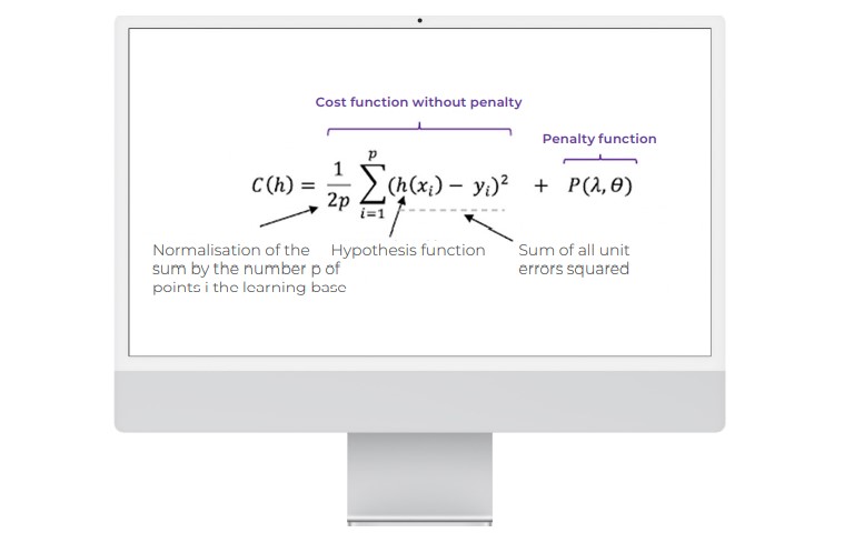
The values of X and Y are given. In terms of its construction, cost function C is a function of the parameters of the hypothesis function (h).

And the parameters of C define an affine line.

This is the function (Penalty function) that manages the penalty according to a lambda parameter which is set empirically in order to obtain the best results.

We suggest that you take a detailed look at three methods based on this principle.

First regularisation method: penalised Ridge regression

Ridge regression is one of the most intuitive penalisation methods. It is used to limit the instability of predictions linked to explanatory variables that are too correlated.

This penalisation function is based on the so-called L2 norm which corresponds to the Euclidean Distance. The Ridge regression is therefore the equivalent of minimising the following cost function:

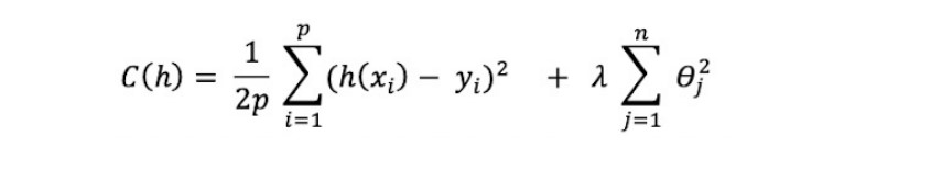
The Ridge penalty will decrease the distance between the possible solutions, based on the Euclidean Measure.

Configuration of the lambda parameter:

• When lambda is near to zero, the classic solution is used, without penalties.
• When lambda is infinite, the penalty is such that all parameters are set to zero.
• When lambda is increased, the bias of the solution is increased, but the variance is reduced (cf. the definition of the bias-variance trade-off).

As with classic linear regression, Ridge regression can be solved by gradient descent, and by iterating until the convergence of cost function C.

Therefore, Ridge regression makes it possible to circumvent problems of collinearity (where explanatory variables are very strongly correlated) in a context where the number of explanatory variables at the input of the problem is high.

The main weakness of this method relates to the difficulties of interpretation because without selection, all the variables are used in the model.

LASSO penalisation method

You might know the term “lasso” from stories about the Wild West. In this context, though, it stands for “Least Absolute Shrinkage and Selection Operator.” The acronym LASSO contains terms relating to the notion of shrinkage of the search space, and other terms relating to a variable selection operation (“selection operator”).

The LASSO method introduces the following penalty term to the cost function formulation:

This time, another norm is used. The L1 norm corresponds to the Manhattan norm (distance corresponding to a movement at right angles on a chessboard – unlike a Euclidean Distance, which corresponds to a movement in a straight line).

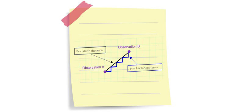
Figure 1 : Distance between two points: Euclidean Distance vs Taxicab Geometry (lots of paths between A and B)

It is a much less intuitive distance than the Euclidean Distance, which allows a penalty and decreases the distance between the possible solutions on the basis of the L1 norm.

The cost function to be minimised by LASSO is written as follows:

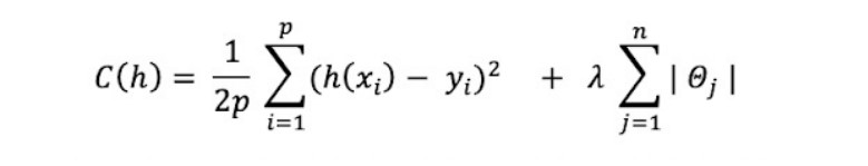
Note that there is no analytical solution for LASSO, and so we can use an iterative algorithm or the gradient descent method to solve this equation.

LASSO does have some good qualities: it is a form of penalisation which makes it possible to set certain coefficients of explanatory variables to zero (unlike Ridge regression, which can lead to coefficients near to 0, but never exactly zero).

LASSO is therefore an algorithm that also allows the simplification of the model, by eliminating variables.

We will now geometrically illustrate the effects of a Ridge Vs LASSO regularisation on the model parameters with the two graphs below.

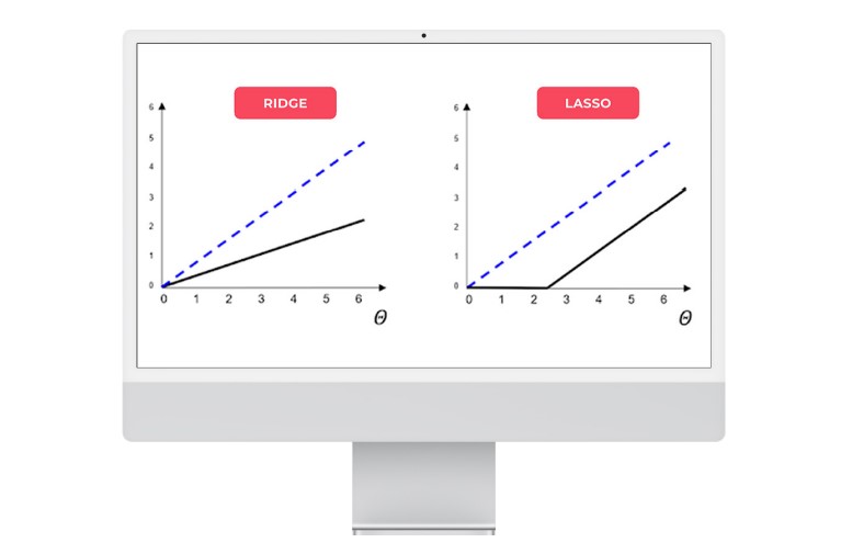
Figure 2: Geometric comparison between Ridge and LASSO regularisation on model parameters

The black line represents the regularisation function, while the dotted blue line represents an unregulated line. It can be seen that the Ridge regression scales the coefficients by dividing them by a constant factor, whereas LASSO subtracts a constant factor by truncating to 0 below a certain value.

Elastic Net = Ridge + LASSO

In practice, Ridge regression gives better results than penalised LASSO regression, especially if the explanatory variables of the problem to be solved are highly correlated (this is the classic use case for this penalisation method).

But Ridge regression does not reduce the number of variables. To find a compromise between the two penalisation techniques, Elastic Net regularisation combines the two approaches.

The cost function is determined:

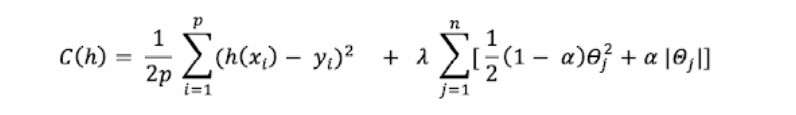
Where the alpha parameter is a parameter defining the balance between Ridge and LASSO.

• For alpha = 1, the cost function matches that of LASSO.
• For alpha = 0, the Ridge regression is found.

It is possible to adjust the penalty depending on the application case.

• When alpha approaches 1, we can have a behaviour near to the LASSO while eliminating the problems relating to strong correlations between explanatory variables.
• When alpha increases from 0 to 1 (for a given lambda), the number of variables removed from the model (leading to a zero coefficient) increases until a smallest model is obtained, obtained by LASSO.

To summarise…

To conclude, regularisation makes it possible to shrink the space formed by the solutions of the modelling problem by linear regression. To do this, we add a term that will penalise the coefficients to the cost function. Minimising the cost function will therefore minimise the regression coefficients.

3 types of regularisation have been presented in this chapter: the Ridge, LASSO and Elastic Net methods.