
Machine learning (ML) models are becoming more and more complex. Indeed, a sophisticated model (e.g. XGBoost boosting or deep learning) generally leads to more accurate predictions than a simple model (e.g. linear regression or decision tree).
There is therefore a trade-off between the performance of a model and its interpretability. What a model gains in performance, it loses in interpretability (conversely).
What exactly is “model interpretability”?
Interpretability is defined as the ability of humans to understand the reasons for a decision made by a model. This criterion has become instrumental for many reasons.
On a scientific level, the development of knowledge and progress depends on a deep understanding of the phenomenon studied. It is therefore unimaginable for a data scientist to let a machine learning model operate without seeking to determine the influential variables, or without aiming to verify the consistency of the results against expert knowledge of the field, etc. It is about understanding, and having confidence in – and proof of – the consistency of the model.
- On an ethical level: let’s imagine a situation where someone is suffering from cancer. They are denied treatment because of the sole decision of an algorithm. Moreover, this algorithm is complex and therefore no surgeon is able to justify such a decision. This situation is not acceptable.
- On a legislative level: Article 22 of the General Data Protection Regulation (GDPR) states that a person must not be the subject of a decision based exclusively on automated processing and emanating solely from the decision of a machine.
In this chapter, we will present two methods with which to interpret machine learning models: the LIME and SHAP algorithms. These two methods operate at the output of a complex model, a black box with poorly understood functioning.
Before looking at the specificities of each algorithm, we suggest that you quickly review what characterises the main interpretability methods.
Interpretability methods
The different interpretability methods can be defined according to the following typologies:
- Agnostic versus specific interpretation methods: Agnostic methods can be used for any type of model. In contrast, specific models can only be used to interpret a specific family of algorithms.
- Intrinsic versus post-hoc methods: In intrinsic methods, interpretability is directly linked to the simplicity of the model; while in post-hoc methods, the model cannot be interpreted because it is too complex from the outset.
- Local versus global methods: Local methods give an interpretation for a single observation, or a small number of them. In contrast, global interpretation methods make it possible to explain all the observations at the same time, globally.
- A priori versus a posteriori methods: A priori approaches are used without assumptions regarding the data, and prior to the creation of the model. In contrast, a posteriori approaches are used after the model has been created.
The current state of the art around the interpretability of machine learning models shows that there is a strong desire to mix the different methods: {intrinsic & global} or {post hoc & global & agnostic} or even { post-hoc & local & agnostic}.
LIME
The LIME algorithm (Local Interpretable Model-agnostic Explanations) is a local model that seeks to explain the prediction of an individual by analysing its surroundings.
LIME has the particularity of being a model:
- Interpretable. It provides a qualitative understanding between the input variables and the response. The input-output relationships are easy to understand.
- Locally simple. The model is globally complex, so it is necessary to look for simpler answers locally.
- Agnostic. It is able to explain any machine learning model.
To do that:
- 1st step: the LIME algorithm generates new data, in a neighbourhood which is near to that of the individual to be explained.
- 2nd step: LIME gives rise to a transparent model on the basis of the predictions of the complex “black box” model that we are trying to interpret. It, therefore, learns using a simple and therefore interpretable model (for example, linear regression or a decision tree).
The transparent model, therefore, acts as a substitute model with
which to interpret the results of the original complex model.
The main drawback of the LIME method relates to its local operation. In addition, LIME does not make it possible to generalise the interpretability resulting from the local model on a more global level.
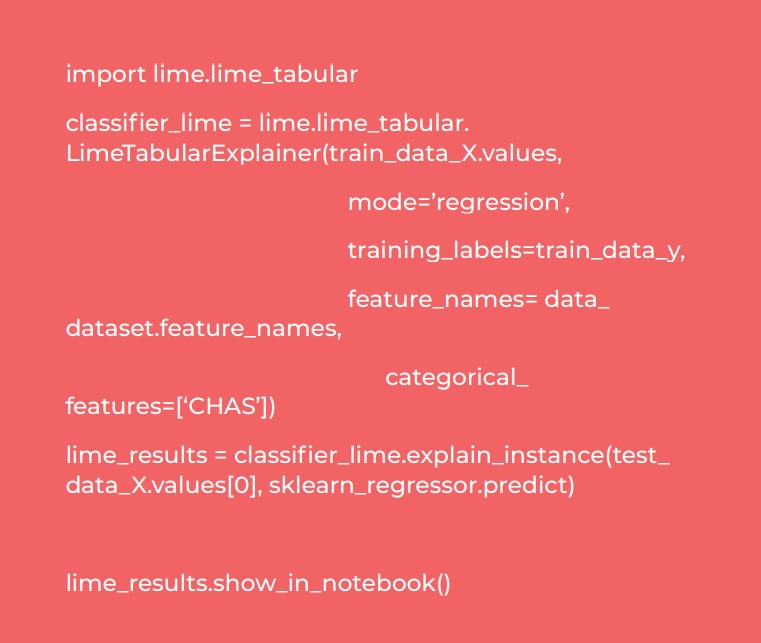
Application with Python
There is a LIME library in Python. According to the input data type, you can use:
- lime.lime_tabular for data tables
- lime.lime_image for image databases
- lime.lime_text for a text corpus.
Our use case: explaining the churn score of a particular customer, based on their transactional data. Different questions need to be asked: How can different score classes be explained? What makes this customer’s score different from those of other customers? What behaviour causes this particular customer to have a certain score?
LIME has enabled us to explain the predictions of a complex XGBoost model, which boosts machine learning.
Results:

The difference in colour shows us which are the favourable and unfavourable factors for the interpretation of the churn:
- in green: favourable factors help to increase the predicted value.
In our example, the customer makes regular purchases. There are no anomalies for this customer.
- in red: unfavourable factors help to increase the customer’s churn risk score.
In our example, the customer has hardly made any purchases in the past week. This should sound a warning – the customer may be losing interest in the brand. In addition, the customer’s lifetime value over the last month is low (€186) compared to their previous purchases. We have to find a way to win them back.
Shap
The implementation of SHAP is based on a method used for estimating Shapley values. There are different estimation methods such as KernelSHAP (a method inspired by LIME) or TreeSHAP (a decision tree-based method).
Shapley value estimation principle
For a given individual, the Shapley value of a variable (or several variables) is its contribution to the difference between the value predicted by the model and the mean of the predictions of all the individuals.
To do that:
- Step 1 in calculating Shapley values for a particular individual: Simulate different combinations of values for the input variables
- Step 2: For each combination, calculate the difference between the predicted value and the average of the predictions. The Shapley value of a variable, therefore, corresponds to the average of the value contribution, according to the various combinations.
Here is a simple example
Imagine that we have created a model for predicting apartment prices in Paris. For a given observation, the model predicts the class “Price > €12,500/m2” with a score of 70% for an apartment with a balcony (presence_balcony variable = 1). When changing the balcony value to 0 (no balcony), the score drops by 20%, and the contribution of the balcony value = 1 is 20%.
Things are indeed more complicated in practice, because to obtain a correct estimate of the Shapley values, we need to add all of the values of each variable of the model, and divide the sum by the number of values in the data set. The calculation time could then become extremely important.
Some lines of Python coding for testing SHAP
In Python, alibi and SHAP libraries implement the methods for estimating the values of Shaply KernelSHAP, TreeSHAP (for use cases on the basis of data tables) and DeepSHAP (for deep learning use cases).
import shap
classifier_shap = shap.KernelExplainer(sklearn_
regressor.predict, data_train_X
shap_results = classifier_shap.shap_values(data_
test_X.iloc[0])
shap.waterfall_plot(classifier_shap.expected_
value,shap_values,data_test_X.iloc[0])
To summarize…
In machine learning, it is important to find a fair compromise between a powerful model versus an interpretable model.
With LIME or SHAP, you can make an initially complex model interpretable and therefore promote its adoption by business users. If understanding a model is essential in a scientific process, legal constraints now require that a decision must not be made based solely on the result of an automatic algorithm.
Remember that the SHAP algorithm currently meets the normative requirements imposed by GDPR.
If you are interested in this subject, we invite you to read about other ways of interpreting machine learning models such as: techniques based on the analysis of “ICE and PDP graphs,” so-called “permutation feature Importance,” “counterfactual explanations,” or even “anchors.”

Predictive models which are too complex tend to be penalised. This is not only because they cannot be generalised for specific, real-world situations, but also because they are difficult to interpret. When such interpretability methods are associated, with complex prediction models, their contribution is invaluable. This enable us to avoid the cost of insights that would not be available to commercial decision makers.

